
In the last article, we discussed the linear function and how we use the linear function unknowingly in our day to day lifeas a part of bio math series. In this article, we will study a few mathematical aspects of the linear function along with some basic operations.
The straight-line graph of the linear functions is formed from many points joining together. The position of each data point on the straight line is denoted as (x,y) by X and Y coordinate. The equation of a straight line is,
Y=mX+C
Given a slope, we can find out the value of the constant-C from any one point on the line. Once we have the value of slope and Y-intercept, we can determine the equation of the straight line.
Suppose you want to find the equation for a line that passes through the point (1,2) and has a slope of 3. Therefore the equation of a line is,
Y = mX+C
Where:
m is the slope,
C is the y-intercept or the constant.
In the present case equation for line looks like,
Y=3X+C.
Now let’s calculate the value of Y intercept, or constant -C of the straight line equation /linear function.
We have point (x,y) as (1,2). This means, the value of the X coordinate of the point is 1 and the same for Y is 2. Because the point falls on the line, we can solve the straight-line equation for C with the mentioned values of X and Y (1,2).
Y=mX+C or 2=3 × 1+C or C=2-(3)(1).
therefore C=-1.
Thus the equation of the line that is passing through the point (1,2) with a slope of 3 is
Y=3X-1.
Whenever we have the non-zero value of the Y-intercept, the line does not pass through the origin.
Deriving equation of line in linear functions
For a linear function the slope m, of the line can be calculated by using the following formula provided we are given Y and Y coordinates of at least two points on the line.
We can determine the equation of a line if we are given two points((X1, Y1), (X2, Y2)) through Which the line is passing. First of all, we must calculate the slope by using the coordinates of two points on the line. Then the Y-intercept can be determined by using coordinates of any of the two points on the straight line and a slope.

This formula basically calculates the rise or drop in the Y values per unit value of X. Slope is also referred to as, rise per run or simply as rate. After substituting the values of all components of the straight-line equations at the right place, we get the equation of that line.
This information of the mathematical operation of the linear function is available in every mathematical textbook but skilful use of mathematics in science is a matter of training. We will now see how linear function work in math and science and also in biology.
In the following example, the height of the plant has been measured over the years. The graph of an increase in the plant height over the period is a straight line which means it is following the linear function.
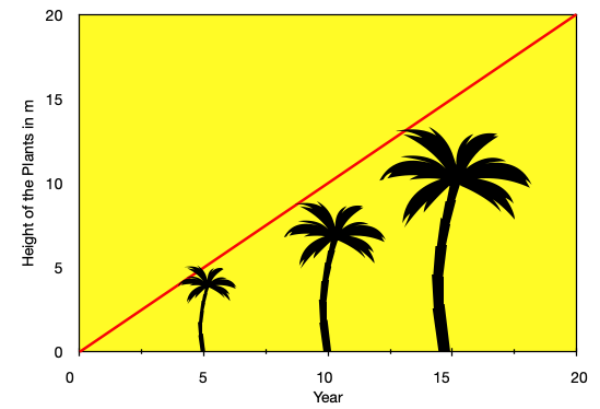
The straight-line equation for the increase in the plant height over the period is,
H=mX+C,
Here Y=H,
Here slope m=1, X=period, and C= Y-intercept or Initial height of the seedling (at the time of zero years) .
The height for the just planted tree is zero therefore there is no Y-intercept, hence no C is present in the equation or it can be considered as zero. That is why the line will pass through the origin. By using this equation we can predict the height of the plant after any number of the years.
For example, after 25 years the height of the plant would be the H= 1×25+0= 25.
One of the major and frequent uses of the linear function is in determining the melting temperature (Tm) of the DNA. The strands of the nucleic acids in the DNA are held together by hydrogen bonding. These hydrogen bonds contribute to the Tm of the DNA fragments. Tm values have numerous applications in PCR technology, Southern blotting, in-situ hybridization, etc. The GC content significantly affects the Tm of the DNA fragments.
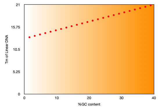
In this graph (designed for only demonstration purpose) we can see that, Tm values for different %GC values form a graph of a straight line.
The equation for Tm can be written as.
Tm=0.2x+13,
where X values are %GC content of the given DNA fragment.
We can use this equation to calculate Tm values for any DNA fragment containing differential %GC composition. There are numerous other are examples of the use of the linear function in biology.
In enzyme kinetics, the rate of product formation by an enzyme or the velocity of the enzyme is calculated by using the plot of product concentration vs the time of reaction. Monomeric enzymes follow the linear increase in product formation.
The spectrophotometric estimation techniques are based on the linear function. We will uncover multiple ways how science math is essential for biological studies in the next articles, we will talk about the importance of the power function and how it is useful in biological study.
